Introduction

This small project aims to present how can we leverage Deep Learning capabilities for 2D texture synthesis, a subdomain of generative AI targetting to generate a texture of any size imitating the style a given one. In this article, I suppose that you are familiar with the terms describing a Neural Network architecture.

We use a VGG-19 neural network [4], a convolutional network architecture used for image classification and pre-trained on ImageNet dataset [1], a large hierarchically database containing more than 14 millions images and more than 20000 label categories. Note that we could also use other networks like ResNet50, which is faster to train and avoids the vanishing gradient problem, but here we choose VGG-19 for the simplicity of its architecture.

What is the style of an image

If you are in front of a Seurat painting (figure 2), you can easily recognize the style. Points everywhere. The style thus seems to dwell in small details, like in the brush stroke itself, not in what it represents. Gatys et al. [2], in their famous style transfer paper, were the first to use Gram Matrices to represent the style of an image. Here is the formula of the gram matrix G for an input image u:

$\large G(u) = \frac{1}{HWD} \phi(u)\phi^ (u)$

Equation 1: Gram Matrix equation

The correlation between the horizontal and vertical features is made by a matrix product between the matrix and its transposed, respectively φ(u) and φT (u) in equation 1. We also normalize the resulting gram matrix by dividing by its dimensions (HW D in equation 1). Since it computes the correlation between the vertical and horizontal information, the gram matrix of an image and its symmetry will give the same result.

More trivially, the gram matrix is a mishmash of a given matrix. Applied to our Seurat painting, we understand that 1 will tear appart the man and its moustache. If you calculate the gram matrices for each image given by a convolution output, you can build a valid representation of the style for different scales (brush hair shape, brush stroke, contours…) without giving importance to macroscopic shapes.

Outline

We will base our work on the method described in [5]. The first step works as follow:
• We pass a source texture as input to the VGG-19 network
• We retrieve the outputs from intermediate layers after each pooling layer. These outputs are called feature
maps.
• We calculate the gram matrices of these feature maps

Subsequently, we introduce a second network Gθ that generates an output image Gθ (z) from an input multi-scale random noise image z. Passing the random image z through the VGG network, we retrieve their correspondent feature maps and we calculate the gram matrices as equation 1. Afterwards, we calculate the mean square error,

$\large \min_\theta \mathbb{E}_{z\sim Z} \sum_l \| \Phi_l(G_\theta(z))-\Phi_l(s) \| _2^2 ,$

Equation 2: Mean square error between the gram matrices of our source texture and our synthesized one.

between the generated image gram matrices Φl(Gθ (z)) and the texture source gram matrices Φl(s). This is the loss we try minimize.

Feeding the input texture to VGG-19

In order to reproduce the image results shown in this article, we manually set a pytorch random seed with the value of 69 using pytorch function:

torch.manual_seed(69)

We choose to train our model for 2000 epochs as in paper [5], using “Adam” optimizer [3], with a learning rate of 0.1 and batch size of 10 samples per epoch. Input texture images were re-scaled into a dimension of 256×256 pixels.

These are the obtained sizes when do a forward pass through the VGG network :

torch.Size([1, 64, 64, 64])
torch.Size([1, 128, 32, 32])
torch.Size([1, 256, 16, 16])
torch.Size([1, 512, 8, 8])
torch.Size([1, 512, 4, 4])

Figure 3: Obtained feature sizes

The features sizes in figure 3 correspond to the output feature size after each MaxPooling/AvgPooling layer of VGG network, as explained in section 1. These are the intermediate layers outputs of VGG-19.

We can appreciate in figure 4 that VGG-19 receives an input image shaped as (1x3x64x64). 1 sample, 3 channels (RGB) and 64 pixels of width and 64 pixels of height.

Then we have a Convolution layer (Conv2d-1) which has 64 filters of size 3×3. This layer has an output of (1x64x64x64). 1 Sample, 64 channels (1 channel per filter) and a dimension of 64×64.

Convolution layer applies padding to the input image before performing the convolution in order to keep the same input size.

After that, we have an Average Pooling 2d layer that reduces the input image of a two factor. Thus, our input size tensor is transformed from 1x64x64x64 to 1x64x32x32.

Then, a second Convolution layer (Conv2d-4) with 128 filters is going to transform the input tensor from 1x64x32x32 into a tensor of shape 1x128x32x32. As we explained before, the size of the output tensor is modified by the number of filters in the convolution layer.

A third convolution and Average pooling 2d layers are applied to our tensor converting it from 1x128x32x32 to 1x256x16x16.

And finally we apply two more convolution – average pooling layers converting into 1x256x16x16 to 1x512x8x8 and a last average pooling to pass into 1x512x4x4.

Calculating the Gram Matrix

As we compute the gram matrix for different layers of the VGG network, we extract different level of details of the style for increasingly deep layers, due to the max pooling.

Here is the gram matrix formula in our method:

$\large \Phi_l(u) = \frac{1}{H_lW_lD_l} \phi_l(u)\phi_l^T(u)$

Equation 3: the gram matrix between the source and synthesized textures for a specific depth l.

Equation 3 is the same than equation 1, except that it depends on the depth of the feature map (hence the
$l$ standing for layer).
As we said in the introduction, during the training, we try to minimize the mean square error between the
gram matrix of the given texture image’s features and that of the generated image.

Time to train!

Let’s start from a peppers texture (the one just above) and see what our network generates.

We observe on the figure 5 that, starting from a mixture of the given texture, the image presents individual peppers at epoch 500.

As we generate a new texture at each epoch from a random noise, it is normal to see some artifacts on the loss curve, as shows figure 6. However, the loss decreases constantly throughout the training, which means the style of the synthesized texture and that of peppers.png becomes increasingly similar.

As we can see on the figure 7, as the network learned the style of our input image (peppers.jpg), we can now synthesize a texture of any size we want. Nevertheless the results are not perfect as we can see green spots artifacts in some peppers.

More results

Let’s try a quite different texture, bones.jpg.

This method [5] does not seem to perform well for bones.jpg (figure 9). As we can see in figure 10, showing the evolution of synthesized images, the resulting generated texture do not converge into the pattern of figure 9. It is likely that the skulls are simply too big to be catched by the gram matrices. A solution could be to artificially de-zoom by repeating this pattern and play with the hyper parameters.

Seeing these results, we got the intuition that this method works better when the texture involves small, randomly-oriented and repetitive patterns. To prove it, we tried to synthesize two textures, one based on a detail of a leaf (with its veins), and one based on a lot of leaves (c.f. figure 11).

Here are the two synthesized textures :

The figure 12 is quite a fail, but the figure 13 looks much more natural. We suppose that the latest contains a lot of examples of leaves, and thus it is easier to generalize.

Different loss functions

Lets try training our model with different loss functions. For this work we compare two models trained on raddish.jpg. One model has been trained using mean squared error loss (L2 distance) and the other one has been trained using mean absolute error (L1 distance).

As we can see in figure 14, both models converge at similar speed and give valid results from epoch 1500.

In figure 15 we compare our models on large texture generation. The left image looks like having a bias that produces diagonal patterns and the model using L2 norm loss produces less biased results. The quadratic nature of L2 implies a higher error sensitivity which explains the absence of bias compared to L1.

Comparing learning loss curves in figure 16 we can appreciate that the L2 loss (right figure) goes down into 10−5 values and the L1 loss barely fall down the 10−3 barrier. Basing on the above results, L2 loss seems to perform better to the problem of texture generation.

Different layers

We tested our network only taking only the first ReLu layer (“r11”) features maps of VGG-19 network.

As we can see in figure 17 we are not capable of exploiting the features of the bones.jpg texture. Besides, the interest of taking the max pooling is to keep the most valuable features of the input image, even so we could extract the main brown color of the source texture image.

Conclusion

After exploring this deep learning approached generative texture method, we can conclude that the method presented in [5] performs very well in texture generation with a highly repetitive pattern.

Furthermore the choice of loss function seems to have a direct impact on the bias of the generated image.

As shown in figure 15, using L2 loss produces more natural and less biased texture patterns that using L1 loss.

At last, we have shown in section 7.2 the importance of every feature map to catch the different level details of a given texture.

References

[1] Jia Deng, Wei Dong, Richard Socher, Li-Jia Li, Kai Li, and Li Fei-Fei. Imagenet: A large-scale hierarchical
image database. pages 248–255, 2009.

[2] Leon A. Gatys, Alexander S. Ecker, and Matthias Bethge. A neural algorithm of artistic style. CoRR,
abs/1508.06576, 2015.

[3] Diederik P. Kingma and Jimmy Ba. Adam: A method for stochastic optimization, 2014. cite
arxiv:1412.6980Comment: Published as a conference paper at the 3rd International Conference for Learning
Representations, San Diego, 2015.

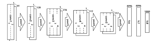
[4] Karen Simonyan and Andrew Zisserman. Very deep convolutional networks for large-scale image recognition.
In Yoshua Bengio and Yann LeCun, editors, 3rd International Conference on Learning Representations,
ICLR 2015, San Diego, CA, USA, May 7-9, 2015, Conference Track Proceedings, 2015.

[5] Dmitry Ulyanov, Vadim Lebedev, Andrea Vedaldi, and Victor S. Lempitsky. Texture networks: Feed-forward
synthesis of textures and stylized images. CoRR, abs/1603.03417, 2016.

Using deep learning for texture synthesis